
Thermo-Economic Optimization of Heliostat Field Distribution Considering Magnitude and Aspect Ratio of Heliostat Using Multiobjective Gray Wolf Optimizer (Case Study: Tehran)
Abstract
This study aims to investigate the effect of heliostat geometry on the performance of a heliostat field. Rectangular reflectors, as a prevalent type of heliostats, were surveyed. The heliostat's aspect ratio significantly affects the shading and blocking factors, ultimately altering the optical efficiency of the heliostat field. The Multiobjective Gray Wolf Optimizer (MOGWO) is used to design a heliostat field composed of heliostats with optimal aspect ratios. The goal is to achieve maximum optical efficiency with the lowest Levelised Cost Of Energy (LCOE). The results indicate that optimizing the heliostat aspect ratio alone increases optical efficiency by 5.2%. However, the simultaneous optimization of the reflectors and the heliostat field can improve optical efficiency by 11%.
Keywords:Heliostat fieldOptical efficiencyThermo-economic optimizationMultiobjective gray wolf optimizer
1. Introduction
Solar energy, as a renewable energy source, is one of the acceptable solutions to reduce the consumption of natural gas and fossil fuels. The share of solar energy in global energy generation increased from 0.01% in 2004 to 1.05% in 2015. Numerous power plants are under construction worldwide [1]. Concentrated solar power is considered one of the most promising among solar energy technologies. It is expected that CSP could supply approximately 11% of the world's electricity needs by 2050 [2]. Over the past decades, Solar Power Tower (SPT) technology has been overtaking other technologies due to higher efficiency and ease of scaling [3]. A classic solar tower power system consists of a solar tower, receiver, power generation parts, and thousands of giant mirrors called heliostats. The power plant usually incorporates energy storage [4]. The heliostat field accounts for about 50% of the overall cost and 40% of the system's energy losses [5], [6]. Consequently, several studies were conducted, and many codes and algorithms, such as Hflcal [7], Mirval [8], Delsol [9], Campo [10], and Hfld [11], were developed to simulate the optical efficiency of the heliostat field. Suhil Kiwan[12] proposed a spiral distribution heliostat field layout with extended typical domains of the shape factors. The PSO algorithm is used to maximize the annual weighted efficiency of a 50 MWth SPT in Ma'an, Jordan. The sensitivity of annual efficiency to the shape factors and the angular position of heliostats was determined. An alternating direction method utilized by Seonghyeok Kiwan and Khammash [13] incorporated the proposed physics-based gradient of optical efficiencies to optimize a pattern-free heliostat field and a scaling factor (k) to generate the initial layout. Recently, particular attention was paid to comparing the biomimetic spiral and radial-staggered layouts.
Zhang et al. [14] developed a rapid, accurate code to determine the optical efficiency of the aforementioned layouts. The results showed better performance of the spiral layout in the north field, since in the circular and southern square, the radial-staggered arrangement was more prosperous. Thermal and economical comparative analyses of Campo radial-staggered and biomimetic spiral layouts were carried out by Gadalla and Saghafifar [15]. Annual weighted efficiency, annual unweighted efficiency, and Levelised Cost of Energy (LCOE) were considered objective functions. Mirror size, the height of the central tower, the number of heliostats in the field, and receiver's dimensions were examined as design variables. Due to the effect of mirror geometry on efficiency, numerous heliostat shapes were surveyed by Belaid et al. [16] to obtain the optimal efficiency of the heliostat field in both layouts. The highest efficiency and lowest land area occurred in Campo radial-staggered layout by using Grasshopper Optimization Algorithm. On the other hand, the implementation of circular heliostats caused the reduction of land area.
The strong dependence of optical efficiency on numerous parameters has complicated heliostat field modeling. The optical efficiency can be affected by the size, shape, and configuration of each component. In addition, the environmental and economic conditions at the power plant construction site strongly affect efficiency [12]. Given the impact of these factors, several studies have been conducted to enhance heliostat field efficiency and reduce LCOE. The wind load effect on heliostats with different pedestal heights was analyzed experimentally [17], [18], and a mathematical model was developed. Lee and Lee [1] analyzed the effects of site slope at various latitudes and discovered the optimal site type. Eventually, the most efficient heliostat field layout was achieved based on the optimal site slope. SolarPILOT was extended and developed by Agarwal et al. [19] to design a heliostat field on hilly terrain. Inspection results of shading and blocking profiles reveal that 10% to 30% of heliostats remain unused during more than half of operating hours due to shading or blocking. Eliminating inefficient heliostats can lead to significant cost reductions.
Several methods have recently emerged due to the difficulty and time-consuming nature of simulating and optimizing the heliostat's desired objective function. Genetic algorithm with a new crossover strategy [20], Multiobjective Particle Swarm Optimization (MOPSO) [21], Hybrid PSO-GA algorithm (a combination of GA and PSO) [2], Gray Wolf optimization (GWO) [22], and a hybrid algorithm combining particle swarm optimization algorithm and genetic algorithm [23] are just a limited number of multiple developed algorithms. Different metaheuristic algorithms, including the Genetic algorithm, differential evolution, particle swarm optimization, grey wolf optimization, improved grey wolf optimization, artificial bee colony, and grasshopper optimization algorithm, were assessed by Arrif et al. [24] to optimize a PS10 plant with a staggered heliostat field. The annual weighted efficiency, used as the objective function, was comprehensively investigated, and several factors, including LCOE, land-use factor, and computational cost, were also examined. The findings indicate that evolutionary algorithms outperform crowd intelligence algorithms in terms of optimization efficiency, while Grasshopper Optimization Algorithm (GOA) and Grey Wolf Optimizer (GWO) are more convergent algorithms.
The spectacular effect of mirror geometry in concentrating sunlight has led to the investigation of diverse mirror shapes. Curved Heliostat Profiles and hexagonal reflectors are just some of the types of mirrors used. However, the effect of utilizing multi-reflector mirrors, unequal heliostats, and umbrella-like support structures instead of traditional T-shaped heliostats on the optical efficiency of the heliostat field has been studied separately [25–30]. Using the GOA, mirrors with circular, octagonal, heptagonal, hexagonal, pentagonal, and square shapes in biomimetic spiral and campo radial-staggered layouts have been optimized to achieve higher efficiency and reduced occupied area [16]. A parametric study of the effect of heliostat aspect ratio on heliostat field cost was conducted by Singhai et al. [31]. Based on the results, the heliostat with an aspect ratio of about 2 is more efficient and economical. Based on the location of the heliostat field and the technologies used, the author suggests further studies in this field. Despite these studies, the optimal heliostat size, balancing efficiency and cost, remains to be determined [32].
Based on the literature review, although various heliostat shapes have been investigated, the appropriate mirror size as an objective function has not been adequately addressed. On the other hand, optical efficiency and LCOE are not optimized simultaneously. The uniqueness of this study lies in its focus on the heliostat aspect ratio as a design parameter to achieve optimal efficiency and LCOE. Another innovation is the multiobjective optimization of the heliostat field arrangement, with optical efficiency and LCOE as objective functions. The Multiobjective Gray Wolf Optimizer (MOGWO) is used to expand the optimal heliostat layout with the best mirror size. This algorithm is used for the first time to optimize the heliostat field in a multiobjective setting.
2. Mathematical Model
A mathematical model was developed to optimize the Campo radial-staggered configuration in two fundamental segments, generating an initial heliostat field and calculating the optical efficiency. The basic system parameters are described in Table 1.
Table 1. Basic parameters for heliostat field [33], [34].
This table is shown in the PDF version of the article.
2.1 Initial Heliostat Field
The primary arrangement of the radial staggered layout was established on the Campo model, as detailed by Collado [10]. In this configuration, the heliostats are arranged on concentric circles, with the central receiver at their center. To reduce shading and blocking effects, heliostats in consecutive rows have different azimuth angles, so that each heliostat is placed between the front-ring heliostats. Fig. 1 depicts the variables used to characterize the heliostat field layout.
This figure is shown in the PDF version of the article.
The distance between the centers of contiguous heliostats represents the characteristic diameter of the heliostat indicated by DM [10].
DM = DH + dsep. (1)
DH = √1 + x2. LH. (2)
LW
x = . (3)
LH
dsep = y. LH, (4)
where dsep states any additional separation distance between adjacent heliostats, LH and LW are the height and width of the heliostat, respectively. X expresses one of the optimization parameters to control the area of heliostats, and Y represents another optimization parameter to adjust the azimuth angle between heliostats. The minimum radial increment is as follows [10]:
ΔRmin = DMcos30 − h ≅ DMcos30. (5)
For the convenience of calculation, the amount of h is neglected due to the small value of DM compared to R1 (the radius of the first row) Zi is introduced as the subsequent optimization parameter to set the radial distance between rings. The i index refers to the zone number where the heliostat is located [2].
ΔRi = ZiDMcos30. (6)
The azimuth angle between two consecutive heliostats in each zone remains constant and is given by Eq. (7) [2], [10].
Δa1 = 2sin−1(DM⁄2R ) ≅ DM⁄R1. (7)
Considering the constancy of the heliostats in a ring in each zone, the azimuth angular distance between adjacent heliostats is expanded incrementally to the point where a heliostat can be placed between them. By replacing a heliostat in the unoccupied space, the next zone is formed, thus the azimuth angle in the later zones can be stated by Eqs. (8) and (9) [10].
Δa2 = Δa1⁄2. (8) Δa3 = Δa1⁄4. (9)
The number of rows in each zone and the number of heliostats per row can be calculated using Eqs. (10) and (11) [10].
Nrowsi = round (2i−1(R1⁄∆Rmin)) i = 1,2,3. (10) Nheli = 2iπRi⁄DM i = 1,2,3. (11)
The radius of the first ring of every zone can then be determined as Eq. (12) [34].
Ri = max ((2Ri−1), (Ri−1 + (Nrowsi−1 − 1)x2,i−1∆Rmin + x2,i−1∆Rmin)) i = 1,2,3. (12)
Finally, the land area occupied by the heliostats is obtained by Eq. (13) [34].
ALand = π(Rlast + 0.5DM)2. (13)
2.2 Optical Efficiency
The instantaneous optical efficiency of a heliostat depends on time and location and is given by Eq. (14) [10].
ηopt(x, y, t) = ρfcos(x, y, t)fatm(x, y)fint(x, y)fsb(x, y, t), (14)
where ρ is the reflectivity of the heliostats, fcos indicates the cosine factor, fat expresses the atmospheric attenuation factor, fitc represents the interception factor or spillage factor, and fsb shows the shading and blocking factor. Fig. 2 depicts a schematic of optical losses.
This figure is shown in the PDF version of the article.
2.2.1 Cosine factor
The cosine factor is expressed as the cosine of the angle between the incident sun rays and the normal vector to the heliostat surface. It can be calculated as the dot product of the unit vector [23].
ηcos = n ⃗ . s. (15)
The azimuth angle, the altitude angle of the sun, and the day and hour at which the calculations are made determine the sun's position in the sky. Atif and Al-Sulaiman [35] comprehensively demonstrates the calculation of the sun vector and the heliostat position vector.
2.2.2 Atmospheric attenuation factor
Atmospheric attenuation accounts for the beam losses of the reflected ray due to scattering by atmospheric molecules. Increasing the distance between the heliostat and the central receiver further increases radiation losses. The calculation is presented in Eq. (16).
fatm = {0 exp .99321 (−0.− 0001106 0.00176.D .D)+1.97×10−8.D2 D D ≤ > 1000m 1000m. (16)
2.3 Validation of Optical Efficiency
The obtained results are validated against the outcomes reported in Refs. [22], [33] and [10]. The comparison results listed in Table 2 emphasize a close match. Also, according to Fig. 3, each heliostat's shading and blocking efficiency is consistent with the Collado efficiency [10].
Table 2. The comparison of the efficiency terms.
This table is shown in the PDF version of the article.
This figure is shown in the PDF version of the article.
2.4 Levelized Cost of Energy
The LCOE is considered for the enhancement of economic performance. LCOE can be stated by Eq. (22) [29].
i[1 + i]nopr [[ nopr ] + rins]Zmir + Zwire + ZLand + Zopr + Zmai
[1 + i] − 1 (22)
LCOE = .
Enet Zmir is taken here to include the heliostat costs and can be calculated by the following equation [29], [44].
Zhelk,i = Fhelk,iAhelk,iNhelk,i. (23)
1 3000
Fhelk,i = 40 + 11.44(Ahel)2 + . (24)
Ahel
Nzone Nrowk
Zmir = ∑ ∑ Zhelk,i. (25)
k=1 i=1
ZLand and Zwire represent the land charge and wiring costs, respectively, which equations can define. (25) and (26) [9], [21], [45].
ZLand = 0.62(1.5ALand + 1.8 × 10⁵). (26)
cell Ahel Nhel,cell,iAhel
Zwire = ∑ Nhel,cell,i [0.031rcell,i + 24 ], ρcell,i = . (27)
i=1 √ρcell,i Acell,i The maintenance cost is considered equivalent to 3% of the initial capital costs, and annual water consumption for mirror washing determines the operating cost, calculated using the following equation, according to the US Department of energy report [46].
Vw,mw = 0.05AhelNhel. (28)
Enet is the annual thermal energy provided by the field regardless of the occurring losses in the receiver [47]. All design variables for the economic model are tabulated in Table 3.
Table 3. The design variables for the economic model.
This table is shown in the PDF version of the article.
3. Multiobjective Optimization
3.1 Establishment of the Objective Function
Optimizing a heliostat field typically involves two primary factors: the daily-average annual optical efficiency and the LCOE. The inherently time-consuming nature of the daily-averaged annual optical efficiency calculations led Al-Suleiman to suggest monthly-averaged annual optical efficiency as an alternative. Given the same results, the monthly-averaged annual optical efficiency served as the first objective function in this study.
12 t=sunset
∑j=1 ∫t=sunrise noptdt
nmaa = t=sunset . (29)
∑12 j=1 ∫t=sunrise dt LCOE is the previously defined objective function.
3.2 Multiobjective Grey Wolf Optimizer
The GWO is a recent metaheuristic optimization algorithm proposed by Mirjalili et al. [48], inspired by the hierarchy and hunting behavior of gray wolves. Later, Mirjalili [49] proposed the multiobjective version to optimize multi-criterion problems in 2016. GWO is used to solve various energy problems [50–53], including the heliostat field.
Xie et al. [22] recommended the GWO for multiobjective purposes in the heliostat field. As demonstrated by Arrif et al. [24], GWO delivers the best optimization results among swarm intelligence algorithms and is considered a fast-converging method.
Hierarchy in gray wolves involves four main orders. Alpha wolves, consisting of a male and a female, act as pack leaders and make key decisions. Beta wolves are ranked second, helping alpha wolves make decisions. Betas obey alpha wolves and command other wolves. The lowest category includes omega wolves.
Although these wolves seem insignificant, the loss of Omega can lead to conflicts and internal problems. If a wolf does not fit into any of these classifications, it is a delta wolf. Delta is considered a mid-range wolf, superior to omega wolves despite obeying the alpha and Beta [48].
In mathematical modeling, the fittest solution is defined as alpha, and Beta and Delta are the next classifications. α, β, and δ are the leaders in finding the optimal solution, and the wolves ω follow these groups in the objective space. The following equations describe the model [48]:
⃗D ⃗ α = |⃗C1. ⃗X ⃗ a − ⃗X ⃗ |. (30) ⃗D ⃗ β = |⃗C2. ⃗X ⃗ β − ⃗X ⃗ |. (31)
⃗D ⃗ δ = |⃗C3. ⃗X ⃗ δ − ⃗X ⃗ |. (32)
⃗X ⃗ 1 = ⃗X ⃗ ∝ − ⃗A ⃗ 1. (⃗D ⃗ ∝). (33)
⃗X ⃗ 2 = ⃗X ⃗ β − ⃗A ⃗ 2. (⃗D ⃗ β). (34)
⃗X ⃗ 3 = ⃗X ⃗ δ − ⃗A ⃗ 3. (⃗D ⃗ δ). (35)
⃗X ⃗ 1 + ⃗X ⃗ 2 + ⃗X ⃗ 3
⃗X ⃗ (t + 1) = . (36)
In multiobjective optimization, an archive of non-dominated solutions from past iterations is maintained, and alpha, Beta, and delta are selected as the leaders of the hunting process.
3.3 Decision-Making in the Multiobjective Optimization
The Pareto-optimal front provides a set of optimal solutions. Therefore, any point in this diagram can be an optimal solution according to the design conditions. However, various methods have been proposed to find the optimal solution on the Pareto frontier so far. Bellman–Zadeh, LINMAP, and TOPSIS are just a limited number of the approaches presented in the fully described [54].
Here, the TOPSIS method is described and implemented. First, the dimensions and scale of the objective function space are normalized as follows [55].
η∗ opt,i = ηopt,i⁄√∑ η2 opt,i i = 1,2, … , n. (37)
LCOEi∗ = LCOEi⁄√∑ LCOEi2 i = 1,2, … , n. (38)
Then, the ideal point is defined as the point at which each objective is optimized. On the other hand, the non-ideal point is the ordinate with the worst value of each objective.
Due to the conflict between the objective functions, these points cannot lie on the Pareto front. The distance of each point on the Pareto front with ideal and non-ideal points (d1 and d2, respectively) specifies the fitness of that solution.
di,+ = √(η∗ opt,i − max(η∗ opt,i)) + (LCOEi∗ − min(LCOEi∗)) i = 1,2, … , n. (39)
di,− = √(η∗ opt,i − max(η∗ opt,i)) + (LCOEi∗ − min(LCOEi∗)) i = 1,2, … , n. (40)
Finally, a closeness parameter is determined as follows:
di,−
Ci = n = 1,2, … , n. (41)
di,+ + di,− The maximum value of Ci can be suggested as the final optimal solution:
di,−
ifinal = i ∈ max ( ) i = 1,2, … , n, (42)
di,+ + di,− where n is the number of points on the Pareto front.
4. Result and Discussion
The GWO algorithm was implemented to survey the heliostat field located in Tehran (52.5 E, 35.7 N). Optical efficiency and LCOE were simultaneously optimized as objective functions. Fig. 4 shows the Pareto front from the optimization, illustrating the trade-off between optical efficiency and LCOE.
The increase in optical efficiency from 57.4% to 61.9% is evident at the expense of increasing LCOE from 23.88 to 33.74. The TOPSIS technique's final solution is marked on the graph. The corresponding contours of optical efficiency, shading, and blocking factor for the selected solutions are depicted in Fig. 5.
This figure is shown in the PDF version of the article.
This figure is shown in the PDF version of the article.
Table 4 illustrates the characteristics of some points, including the TOPSIS solution, the most efficient, and the lowest LCOE point. The optical efficiency reaches a climax at a square shape. By contrast, at the lowest LCOE point, the aspect ratio rises to 2.2747. The least land occupied is suggested by the TOPSIS method, where a 37.5% decrease in LCOE can be achieved in exchange for a 5% decrease in optical efficiency relative to the maximum efficiency point. To recapitulate, the optimal solution occurs in a domain of aspect ratio from 1 to 2.2747, which is inversely proportional to efficiency and directly proportional to LCOE.
Table 4. The features of the selected solution on the Pareto frontier.
This table is shown in the PDF version of the article.
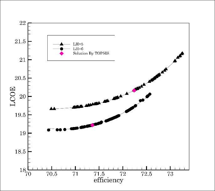
For further investigation, the Pareto front is illustrated at the spring equinox (a), summer solstice (b), autumn equinox (c), and winter solstice (d) with different heliostat lengths in Fig. 6. Despite the variation in the optical efficiency and LCOE, all the graphs have the same behavior. In all cases, increasing the heliostat's length results in a slight decline in optical efficiency. However, it decreases the LCOE in most diagrams, except at the winter solstice, where optical efficiency is lower than on other days. Accordingly, the Pareto front takes place in a larger domain. Table 5 compares the optimal heliostats selected by the TOPSIS method. Optical efficiency and corresponding LCOE are also provided. As shown, the LCOE coefficient remains unchanged despite the leap in optical efficiency as a result of an increase in the length of the heliostat at the winter solstice at the TOPSIS selected solution. Moreover, the results closest in terms of aspect ratio and optical efficiency to annual optimization occur at the winter solstice. That is why the results are presented later at the winter solstice.
Table 5. Comparing the optimal heliostats selected by the TOPSIS method.
This table is shown in the PDF version of the article.
This figure is shown in the PDF version of the article.
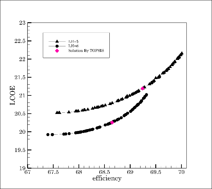
Subsequently, given the responsibility of heliostat length in the final optimal solution, heliostats with constant area were optimized to determine the optimal dimensions. The optimization results determine the domain of aspect ratio. The results are optimized for two cases: 1) Traditional heliostats used in solar power plants and 2) The formerly optimized heliostats. As the patterns in Fig. 7 show, reducing the mirrors' area from the common size to the optimized values increases efficiency. On the contrary, the LCOE declined.
This figure is shown in the PDF version of the article.
Table 6 provides additional specifications for the graphs in Fig. 7. Generally, the aspect ratio of the Pareto front increases as the heliostat area decreases. In contrast, the number of heliostats does not affect the aspect ratio. On the other hand, as the number of heliostats increases, the shading and blocking efficiency decreases, ultimately leading to a decrease in optical efficiency.
Table 6. Comparing the performance of heliostats with different areas.
This table is shown in the PDF version of the article.
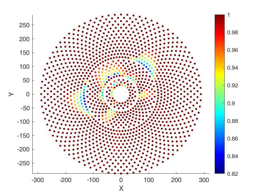
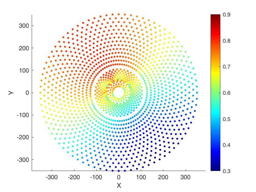
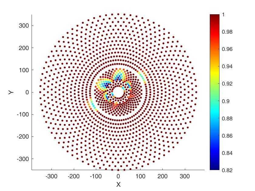
Applying optimum heliostats in a larger solar power plant can significantly improve the performance of the heliostat field. As Table 7 shows, the optical efficiency increased to 44.85% due to a 7% increase in the shading and blocking factor at 10 a.m. on the winter solstice. The thermal energy provided by the field increased by 5.19% after optimization, and a 3.6 decrease in LCOE is evident. On the downside, the field's area expanded to 1680300 m2. It is worth noting that heliostat optimization has been achieved solely by modifying the aspect ratio of the constant-area heliostat. Substituting the optimum heliostats in the optimized heliostat field exceeded the optical efficiency by 11%. Likewise, the thermal energy provided by the field and the LCOE increased by 10% and 6.4%, respectively. Fig. 8 and Fig. 9 show the optical efficiency of each heliostat and the corresponding shading and blocking effect, respectively.
This figure is shown in the PDF version of the article.
This figure is shown in the PDF version of the article.
Table 7. Optimization parameters and comparison of objective functions before and after optimization.
This table is shown in the PDF version of the article.
5. Conclusions
The mirrors' aspect ratio was optimized based on the influence of heliostat geometry on the optical efficiency of the heliostat field. Optical efficiency and LCOE were considered objective functions. The results were optimized using the multiobjective gray wolf algorithm, and Pareto fronts were presented for heliostats with different lengths and varying areas. The ultimate solutions were applied to large solar power plants. Optical efficiency, shading and blocking factor, LCOE, thermal energy provided by the field, and area occupied by the heliostat field were compared. Substitution of heliostats with optimal aspect ratios led to a significant improvement in the performance of the heliostat field, although the construction area of the heliostat field increased noticeably. Since heliostats are generally built in areas with low land value, and given the economic analyses presented in this article, replacing reflectors with optimized dimensions can yield a significant improvement in the performance of the heliostat field in terms of thermodynamics and economics.
Conflict of Interest
The authors declare no conflict of interest.
Data Availability
All data are included in the text.
Funding
This research received no specific grant from funding agencies in the public, commercial, or not-for-profit sectors.
Appendix
Table A1. Nomenclature and symbols used in heliostat field analysis.
Nomenclature Int Interception A Surface area [m2] Land field of heliostat D Distance between the maa monthly averaged annual heliostat center and the aim point in the receiver [m] DH Heliostat diagonal [m] mai Maintenance DM Characteristic diameter [m] mir Mirror dsep Extra security distance [m] opr Operation Enet Annual thermal energy opt optical [MWh] F Heliostat cost per unit area sb Shading and blocking factor [US$/m2] LCOE Levelized Cost Of Energy w Water LH height of the heliostat [m] List of Greek symbols Table A1. Continued.
Nomenclature Int Interception Nomenclature LW width of the heliostat [m] Δai azimuthal spacing between adjacent heliostats in the ith zone n ⃗ unit normal vector of the ΔRi radial distance between heliostat the rows of heliostats in the ith zone, m nopr Field life time cycle ΔRmin minimum radial distance between the rows of heliostats Nhel_i number of heliostats in the ith η Efficiency zone Nrows_i number of rows of heliostats ρ reflectivity of the in the ith zone heliostat Ri radius of first row of heliostat σast standard deviation of of ith zone [m] astigmatic error
s unit vector pointing toward σbd standard deviation of the sun beam quality error Z Capital investment cost [US$] σsun standard deviation of sunshape error Subscript σtot total standard deviation on the receiver plane atm Atmospheric attenuation σtrack standard deviation of tracking error cos Cosine ω incidence angle hel Heliostat
Figures
References
- [1] Lee, K., & Lee, I. (2019). Optimization of a heliostat field site in central receiver systems based on analysis of site slope effect. Solar Energy, 193, 175-183. https://doi.org/10.1016/j.solener.2019.09.027
- [2] Li, C., Zhai, R., Liu, H., Yang, Y., & Wu, H. (2018). Optimization of a heliostat field layout using hybrid PSO-GA algorithm. Applied thermal engineering, 128, 33–41. https://doi.org/10.1016/j.applthermaleng.2017.08.164
- [3] Wang, J., Duan, L., Yang, Y., & Yang, L. (2019). Rapid design of a heliostat field by analytic geometry methods and evaluation of maximum optical efficiency map. Solar energy, 180, 456–467. https://doi.org/10.1016/j.solener.2019.01.052
- [4] Schramek, P., & Mills, D. R. (2003). Multi-tower solar array. Solar energy, 75(3), 249–260. https://doi.org/10.1016/j.solener.2003.07.004
- [5] Rizvi, A. A., Danish, S. N., El-Leathy, A., Al-Ansary, H., & Yang, D. (2021). A review and classification of layouts and optimization techniques used in design of heliostat fields in solar central receiver systems. Solar energy, 218, 296–311. https://www.sciencedirect.com/getaccess/pii/S0038092X21001122/purchase
- [6] Collado, F. J., & Guallar, J. (2019). Quick design of regular heliostat fields for commercial solar tower power plants. Energy, 178, 115–125. https://doi.org/10.1016/j.energy.2019.04.117
- [7] Schwarzbözl, P., Pitz-Paal, R., & Schmitz, M. (2009). Visual HFLCAL-A software tool for layout and optimisation of heliostat fields. In Proceedings. Proceedings. https://elib.dlr.de/60308/
- [8] Leary, P. L., & Hankins, J. D. (1979). User's guide for MIRVAL: A computer code for comparing designs of heliostat-receiver optics for central receiver solar power plants (No. SAND-77-8280). Sandia National Laboratories (SNL-CA), Livermore, CA (United States). https://doi.org/10.2172/6371450
- [9] Kistler, B. L. (1986). A user's manual for DELSOL3: a computer code for calculating the optical performance and optimal system design for solar thermal central receiver plants (No. SAND86-8018). Sandia National Labs., Livermore, CA (USA). https://www.osti.gov/servlets/purl/7228886
- [10] Collado, F. J., & Guallar, J. (2012). Campo: Generation of regular heliostat fields. Renewable energy, 46, 49–59. https://doi.org/10.1016/j.renene.2012.03.011
- [11] Yao, Z., Wang, Z., Lu, Z., & Wei, X. (2009). Modeling and simulation of the pioneer 1 MW solar thermal central receiver system in China. Renewable energy, 34(11), 2437–2446. https://doi.org/10.1016/j.renene.2009.02.022
- [12] Leonardi, E., Pisani, L., Les, I., Larrayoz, A. M., Rohani, S., & Schöttl, P. (2019). Techno-economic heliostat field optimization: Comparative analysis of different layouts. Solar energy, 180, 601–607. https://doi.org/10.1016/j.solener.2019.01.053
- [13] Kiwan, S., & Khammash, A. L. (2018). Investigations into the spiral distribution of the heliostat field in solar central tower system. Solar energy, 164, 25–37. https://doi.org/10.1016/j.solener.2018.02.042
- [14] Zhang, M., Yang, L., Xu, C., & Du, X. (2016). An efficient code to optimize the heliostat field and comparisons between the biomimetic spiral and staggered layout. Renewable energy, 87, 720–730. https://doi.org/10.1016/j.renene.2015.11.015
- [15] Gadalla, M., & Saghafifar, M. (2016). Thermo-economic and comparative analyses of two recently proposed optimization approaches for circular heliostat fields: Campo radial-staggered and biomimetic spiral. Solar energy, 136, 197–209. https://doi.org/10.1016/j.solener.2016.07.006
- [16] Belaid, A., Filali, A., Hassani, S., Arrif, T., Guermoui, M., Gama, A., & Bouakba, M. (2022). Heliostat field optimization and comparisons between biomimetic spiral and radial-staggered layouts for different heliostat shapes. Solar energy, 238, 162–177. https://doi.org/10.1016/j.solener.2022.04.035
- [17] Zang, C., Wang, Z., Liu, H., & Ruan, Y. (2012). Experimental wind load model for heliostats. Applied energy, 93, 444–448. https://doi.org/10.1016/j.apenergy.2011.12.027
- [18] Mammar, M., Djouimaa, S., Gärtner, U., & Hamidat, A. (2018). Wind loads on heliostats of various column heights: An experimental study. Energy, 143, 867–880. https://doi.org/10.1016/j.energy.2017.11.032
- [19] Agarwal, N., Raj, M., & Bhattacharya, J. (2020). Solar tower on an uneven terrain: methodology and case study. Renewable energy, 161, 543–558. https://doi.org/10.1016/j.renene.2020.07.113
- [20] Wang, J., Duan, L., & Yang, Y. (2018). An improvement crossover operation method in genetic algorithm and spatial optimization of heliostat field. Energy, 155, 15–28. https://doi.org/10.1016/j.energy.2018.05.004
- [21] Zhang, H., Bayati, M., Ehyaei, M. A., Ahmadi, A., & Costa, V. A. F. (2021). Optimization of a heliostat field by multiobjective particle swarm optimization (MOPSO) Algorithm based on energy, exergy, and economic point of views. Research Square, 1-42. https://doi.org/10.21203/rs.3.rs-934134/v1
- [22] Xie, Q., Guo, Z., Liu, D., Chen, Z., Shen, Z., & Wang, X. (2021). Optimization of heliostat field distribution based on improved Gray Wolf optimization algorithm. Renewable energy, 176, 447–458. https://doi.org/10.1016/j.renene.2021.05.058
- [23] Li, C., Zhai, R., & Yang, Y. (2017). Optimization of a heliostat field layout on annual basis using a hybrid algorithm combining particle swarm optimization algorithm and genetic algorithm. Energies, 10(11), 1924. https://www.mdpi.com/1996-1073/10/11/1924
- [24] Arrif, T., Hassani, S., Guermoui, M., Sánchez-González, A., Taylor, R. A., & Belaid, A. (2022). GA-GOA hybrid algorithm and comparative study of different metaheuristic population-based algorithms for solar tower heliostat field design. Renewable energy, 192, 745–758. https://doi.org/10.1016/j.renene.2022.04.162
- [25] Landman, W., & Gauché, P. (2012). Sensitivity analysis of a curved heliostat facet profile. SASEC 2016At: Stellenbosch. https://www.researchgate.net/publication/314258829_A_Parametric_Study_of_Heliostat_Size_for_Red uctions_in_Levelized_Cost_of_Electricity
- [26] Schramek, P., & Mills, D. R. (2004). Heliostats for maximum ground coverage. Energy, 29(5–6), 701–713. https://doi.org/10.1016/S0360-5442(03)00178-6
- [27] Hu, Y., Xu, Z., Zhou, C., Du, J., & Yao, Y. (2020). Design and performance analysis of a multi-reflection heliostat field in solar power tower system. Renewable energy, 160, 498–512. https://doi.org/10.1016/j.renene.2020.06.113
- [28] Carrizosa, E., Domínguez-Bravo, C., Fernández-Cara, E., & Quero, M. (2014). An optimization approach to the design of multi-size heliostat fields. Tech. rep., Institute of Mathematics of University of Seville (IMUS)). https://optimization-online.org/wp-content/uploads/2014/05/4372.pdf
- [29] Saghafifar, M., Gadalla, M., & Mohammadi, K. (2019). Thermo-economic analysis and optimization of heliostat fields using AINEH code: Analysis of implementation of non-equal heliostats (AINEH). Renewable energy, 135, 920–935. https://doi.org/10.1016/j.renene.2018.12.060
- [30] Yang, M., Zhang, Y., Wang, Q., Zhu, Y., & Taylor, R. A. (2022). A coupled structural-optical analysis of a novel umbrella heliostat. Solar energy, 231, 880–888. https://doi.org/10.1016/j.solener.2021.12.018
- [31] Singhai, R., Sinhmar, H., & Banker, N. D. (2020). Effect of aspect ratio of heliostat on cost of energy from solar power tower plants. Arabian journal for science and engineering, 45(2), 877–890. https://doi.org/10.1007/s13369-019-04105-0
- [32] Merchán, R. P., Santos, M. J., Medina, A., & Hernández, A. C. (2022). High temperature central tower plants for concentrated solar power: 2021 overview. Renewable and sustainable energy reviews, 155, 111828. https://doi.org/10.1016/j.rser.2021.111828
- [33] Besarati, S. M. (2014). Analysis of advanced supercritical carbon dioxide power cycles for concentrated solar power applications. University of South Florida. https://www.proquest.com/openview/4e1fb9583df75304cac3404dc05b221f/1?pq-origsite=gscholar&cbl=18750
- [34] Huang, W., Li, L., Li, Y., & Han, Z. (2013). Development and evaluation of several models for precise and fast calculations of shading and blocking in heliostats field. Solar energy, 95, 255–264. https://doi.org/10.1016/j.solener.2013.06.016
- [35] Atif, M., & Al-Sulaiman, F. A. (2015). Optimization of heliostat field layout in solar central receiver systems on annual basis using differential evolution algorithm. Energy conversion and management, 95, 1–9. https://doi.org/10.1016/j.enconman.2015.01.089
- [36] Rizvi, A. A., Addoweesh, K., El-Leathy, A., & Al-Ansary, H. (2014). Sun position algorithm for sun tracking applications. In IECON 2014-40th annual conference of the IEEE industrial electronics society (pp. 5595-5598). IEEE. https://doi.org/10.1109/IECON.2014.7049356
- [37] Piroozmand, P., & Boroushaki, M. (2016). A computational method for optimal design of the multi-tower heliostat field considering heliostats interactions. Energy, 106, 240–252. https://doi.org/10.1016/j.energy.2016.03.049
- [38] Huang, W., Li, H., Li, L., Hu, P., & Chen, Z. (2013). Gauss--Legendre integration of an analytical function to calculate the optical efficiency of a heliostat. Solar energy, 92, 7–14. https://doi.org/10.1016/j.solener.2013.03.001
- [39] Lipps, F. W., & Vant-Hull, L. L. (1974). Shading and blocking geometry for a solar tower concentrator with rectangular mirrors. In American society of mechanical engineers, winter annual meeting. https://ui.adsabs.harvard.edu/abs/1974asme.meetS....L/abstract
- [40] Ortega, G., & Rovira, A. (2017). Proposal and analysis of different methodologies for the shading and blocking efficiency in central receivers systems. Solar energy, 144, 475–488. https://doi.org/10.1016/j.solener.2017.01.054
- [41] Rizvi, A. A., & Yang, D. (2022). A detailed account of calculation of shading and blocking factor of a heliostat field. Renewable energy, 181, 292–303. https://doi.org/10.1016/j.renene.2021.09.045
- [42] Besarati, S. M., & Goswami, D. Y. (2014). A computationally efficient method for the design of the heliostat field for solar power tower plant. Renewable energy, 69, 226–232. https://doi.org/10.1016/j.renene.2014.03.043
- [43] Sassi, G. (1983). Some notes on shadow and blockage effects. Solar energy;(United Kingdom), 31(3), 331-
- [333] https://doi.org/10.1016/0038-092X(83)90022-1
- [44] Blackmon, J. B. (2013). Parametric determination of heliostat minimum cost per unit area. Solar energy, 97, 342–349. https://doi.org/10.1016/j.solener.2013.08.032
- [45] Ehyaei, M. A., Ahmadi, A., Assad, M. E. H., & Salameh, T. (2019). Optimization of parabolic through collector (PTC) with multi objective swarm optimization (MOPSO) and energy, exergy and economic analyses. Journal of cleaner production, 234, 285–296. https://doi.org/10.1016/j.jclepro.2019.06.210
- [46] Saghafifar, M., & Gadalla, M. (2016). Thermo-economic analysis of air bottoming cycle hybridization using heliostat field collector: A comparative analysis. Energy, 112, 698–714. https://doi.org/10.1016/j.energy.2016.06.113
- [47] Collado, F. J., & Turégano, J. A. (1989). Calculation of the annual thermal energy supplied by a defined heliostat field. Solar energy, 42(2), 149–165. https://doi.org/10.1016/0038-092X(89)90142-4
- [48] Mirjalili, S., Mirjalili, S. M., & Lewis, A. (2014). Grey wolf optimizer. Advances in engineering software, 69, 46–61. https://doi.org/10.1016/j.advengsoft.2013.12.007
- [49] Mirjalili, S., Saremi, S., Mirjalili, S. M., & Coelho, L. dos S. (2016). Multi-objective grey wolf optimizer: a novel algorithm for multi-criterion optimization. Expert systems with applications, 47, 106–119. https://doi.org/10.1016/j.eswa.2015.10.039
- [50] Li, P., Han, Z., Jia, X., Mei, Z., Han, X., & Wang, Z. (2019). Analysis and comparison on thermodynamic and economic performances of an organic Rankine cycle with constant and one-dimensional dynamic turbine efficiency. Energy conversion and management, 180, 665–679. https://doi.org/10.1016/j.enconman.2018.11.017
- [51] Alirahmi, S. M., Mousavi, S. F., Ahmadi, P., & Arabkoohsar, A. (2021). Soft computing analysis of a compressed air energy storage and SOFC system via different artificial neural network architecture and tri-objective grey wolf optimization. Energy, 236, 121412. https://doi.org/10.1016/j.energy.2021.121412
- [52] Chen, J., Huang, S., & Shahabi, L. (2021). Retracted: Economic and environmental operation of power systems including combined cooling, heating, power and energy storage resources using developed multi-objective grey wolf algorithm. https://doi.org/10.1016/j.apenergy.2021.117257
- [53] Habibollahzade, A., Fakhari, I., Mohsenian, S., Aberoumand, H., & Taylor, R. A. (2021). Multi-objective grey wolf optimization of solar chimneys based on an improved model incorporating a wind turbine power curve. Energy conversion and management, 239, 114231. https://doi.org/10.1016/j.enconman.2021.114231
- [54] Ahmadi, M. H., Mohammadi, A. H., & Dehghani, S. (2013). Evaluation of the maximized power of a regenerative endoreversible Stirling cycle using the thermodynamic analysis. Energy conversion and management, 76, 561–570. https://doi.org/10.1016/j.enconman.2013.07.082
- [55] Wang, K., He, Y.L., Xue, X. D., & Du, B. C. (2017). Multi-objective optimization of the aiming strategy for the solar power tower with a cavity receiver by using the non-dominated sorting genetic algorithm. Applied energy, 205, 399–416. https://doi.org/10.1016/j.apenergy.2017.07.096